


As data scientists, we are responsible for the whole process of implementing machine learning algorithms for the benefit of our customers: from choosing problems and algorithms to follow-up measurement and refinement. After an initial implementation of a new algorithm, we have to watch closely how it performs in real life and quickly iterate together with Product and Software Engineering to eliminate performance bottlenecks and respond to important effects we did not prepare for.
In this post, I will tell a story about how a supposedly minor difference between A/B testing groups can shift a whole experiment.
It started with a routine follow-up of a pilot using the new algorithm, but as more and more days passed, it became apparent that what we saw was not random noise but an important effect we did not yet understand. We brainstormed about possible causes and what we should experience if one of our assumptions was an oversimplification. Then we carefully checked each of these ideas until we understood what was behind the scenes.
The Machine Learning Part
The objective came from our customers: send emails to each of their contacts with the best possible timing when the contacts are the most receptive. We thought about and tested many different approaches and chose a slightly modified multi-armed bayesian bandit algorithm. We decided on sending time based on previous success of different send times. We assume each contact has an open rate in every two-hour slot of the day and they open each email sent in that time slot with this probability. Depending on whether they opened a particular email in the time slot, we update the parameters of the beta distribution of that time slot in a bayesian manner. As time went on we had more information, thus smaller variance in every time slot and with higher and higher probability we would send each letter in the time slot with the highest open rate.
Deciding on one send in detail: we sampled once from each of the 12 beta distributions and chose the slot with the highest sample value. Before each send, we took the one year history of the contact and computed priors based on previous send time optimized campaigns globally. This way we have as much information as possible for new contacts as well. Note that we not only learn from opens, but also from sends without opens as well.
Tendencies We Expected
So the algorithm was optimizing the sending on an hourly basis regardless of the day of the week. However, people have different daily routines on weekends and on weekdays. We have five weekdays competing with two weekend days. Thus we assumed that the algorithm would learn weekday preferences because weekend performance would be worse. We also knew that once the algorithm learned something, it was slow to adapt if preferences changed. It would also easily get stuck in a sub-optimal state if the first few reactions were not typical: either by chance or if a contact gets exceptionally engaging campaigns in sub-optimal or even bad time slots.
In order to see the added value despite the natural fluctuation in campaign open rate we decided to measure results with A/B testing: send emails to the first group with send time optimization and send the other group emails at a fixed time. Then we measured the relative performance of the two groups getting exactly the same email at different times.
From previous experience we knew that different campaigns have a huge variance in their open rate. This is why we chose a series of similar daily campaigns for testing the algorithm. From simulations we could predict that the uplift we could hope for was much less than the effect of content or seasonality for example.
… and those that surprised us
Send time optimized campaigns performed better on weekends better but significantly worse on weekdays. The variance was high but still the pattern was clear.
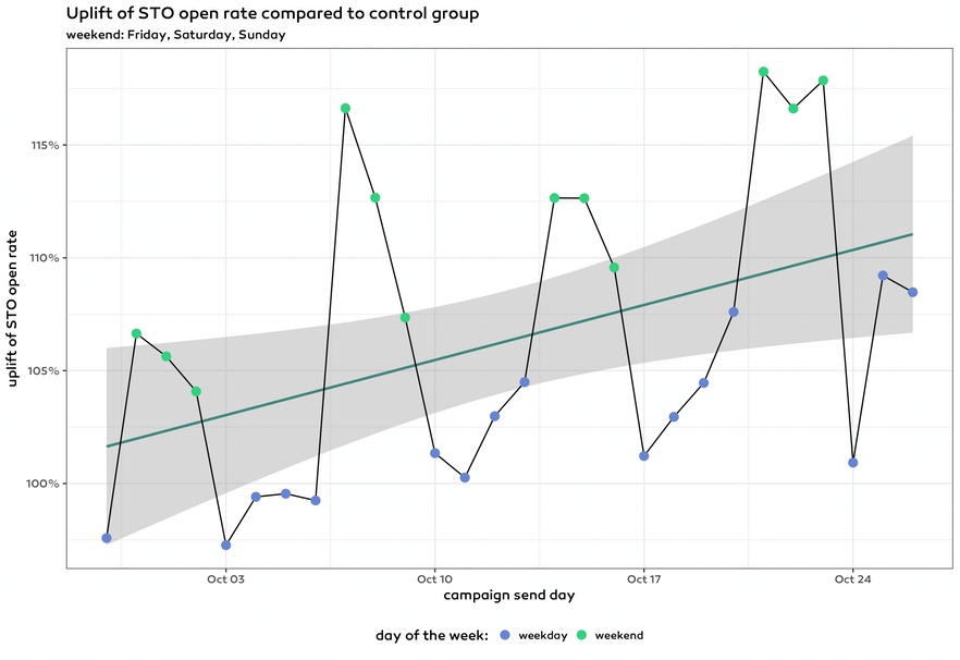
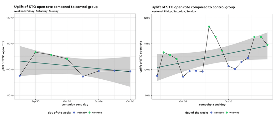
When we looked at the data after one week the overall trend was downwards as on a Thursday in all the data up to that point the effect of weekdays outweighed the effect of weekends. However, if we looked at all the data two weeks later on a Sunday the numbers indicated the underlying upward trend.
The underlying effect
It was not obvious to figure out — since this phenomenon became significant just after a month — that this customer’s globally observed open rate is contrasting on different days of the week. From Monday to Friday the open rate decreases then it picks up again till Monday. Of course the variance is high but by examining the median of campaign open rates on different days the pattern became apparent. There were two more important effects:
- Time optimized sending started in the afternoon and ended next day early afternoon.
- Morning is the best time for most of the contacts.
Combining these two effects most of the contacts in the STO group got their email almost one day later than those in the control group. For example on Tuesdays the open rate of the STO group was attributed to the Tuesday campaign as sending started on Tuesday but actually it reflected the open rate on Wednesday. On the other hand the open rate of the CONTROL group was indeed the open rate on Tuesday as their emails were sent out immediately.

The solution
First and foremost, we wanted to measure our performance from this data as precisely as possible. This was an important pillar of gaining the trust of our client, so keep using the send time optimization feature with a modified setup. We came up with two approaches.
- Compare same days of the week over time. With this approach we have much smaller amount of data but we completely eliminated the problem.
- Aggregate first to weeks and then compare weeks over time. With this approach we either take only weeks with send on all 7 days of the week (not a realistic setup) or remain with some part of the problem. We chose to include weeks with sends on at least 5 days and could see some improvement over time although after aggregation we had few remaining data points.
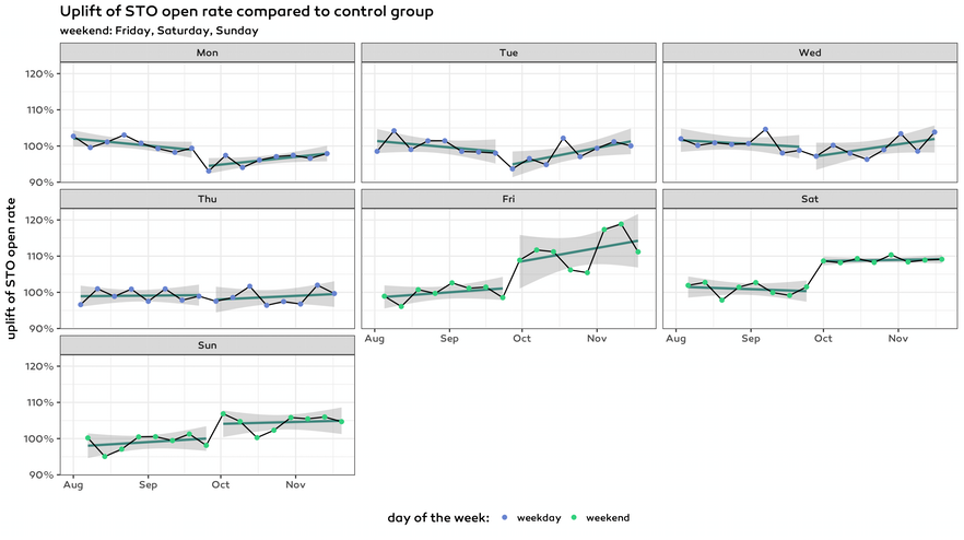
In the above chart we plotted data from 8 weeks before starting to use send time optimization to 8 weeks with send time optimization.
Next, we wanted to ensure that later comparisons are as easy as possible. The most straightforward and easy fix is described below.
Send the emails to the control group in the middle of the time range in which sending to the send time optimized group is spread. Rephrasing this — as usually marketers have a fixed time for sending — set the launch date of the send time optimised group around 12 hours earlier then the launching of the control group campaign. Actually a good compromise is to set the launch date of the send time optimised campaign to midnight as most of the campaigns’ launch times are around 6AM to 6PM. This way it is easier to identify pairs of campaigns later.
Closing thoughts
Own the assumptions of your algorithm and measurement process as real life will always be different from the lab and you want to measure your results, even if you know your model oversimplifies the reality.
Think about alternatives of A/B testing, not only for making decisions but for measuring your existing algorithms as well.
You might have problems either with your machine learning algorithm or with your measurement process: watch out for both!
This post originally appeared on the SAP Engagement Cloud Craftlab blog.